TP R n°1
Normal distribution, random sampling, and dataframe manipulation.
Introduction
For the R practical exercises, you can record your code samples in R scripts, if you want, but you should better write them down in Rmarkdown or Quarto documents. You may want to use an integrated development environment (IDE) such as Rstudio, Positron, or Visual Studio Code with R extensions. Otherwise, any text editor with R code syntax highlighting is sufficient, if you manage the command line.
First step with the R console
- Create a folder for this practical exercise
- Open the R console and use the
setwd()function to move the current R context to a dedicated folder. The
paste0function allows to concatenate strings. The syntax is the following:course <- "R programming" paste0(c("Do you enjoy ", course, "?"))Using the builtin R help command (e.g.,
?paste0), find what is thepaste0function argument that specifies with which character the given strings are joined.Modify the example to concatenate the strings to obtain the string “Do you enjoy R programming?”
Normal law
R includes a large number of builtin functions that make working on statistical analysis rather easy.
The function
rnormallows us to perform a random sampling of the normal law.This function accepts two main arguments, the mean and the standard deviation of the normal distribution.
Use the
rnormfunction to make 100 samples of a variable \(X \sim \mathcal{N}(\mu, \sigma^2)\), where the mean \(\mu = 159.5\) and standard deviation \(\sigma = 10\).Store this sample values into a vector.
- Using the
histfunctions, represent your sampling with the histogram value. Add the density plot of the normal distribution using the following code snippets:
x <- seq(140, 180) plot(x, dnorm(x, mean = mean , sd = sd), type = "l", ylim = c(0, 0.1), ylab = "", lwd = 2, col = "red")- Do you think your histogram does correctly fit the theoretical distribution?
Using the
plotanddnormfunctions, represent on the same plot two Gaussian (normal) distribution \(N_1 \sim \mathcal{N}(\mu = 0, \sigma = 1)\) the reduced and centered normal law, and \(\mathcal{N}(\mu = 19, \sigma = 4)\) variables.You can use the function
linesinstead ofplotsfor the second curve, to add a curve to the plot.You can use the
seqfunction argumentlength.outto increase the resolution.- What happens to the density curve of a normal law when \(\sigma\) increases?
Percentiles
The percentile is the percentage of observations below a given datapoint.
Graphically, the percentile is the area under the probability distribution curve on the left of the observation datapoint.
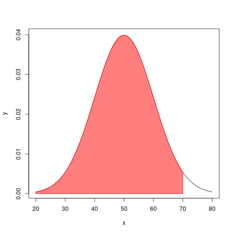
To compute the percentile, we use the function pnorm.
- Compute the percentile of the normal law \(N(\mu = 1500, \sigma^2 = 300)\) of an observation \(x = 1753\).
The 68-95-99.7 “rule”
For a nearly normally distributed data, about 68% of the observations falls within 1 standard deviation (\(\sigma\)) of the mean. About 95% of the observations falls within 2 standard deviations of the mean, and about 99.7% falls with 3 standard deviations of the mean.
Check whether this assertion holds on a random sample of \(n = 125\) observations of the random variable \(X_i \sim N(\mu, \sigma^2)\) where \(\mu = 1986\), \(\sigma^2 = 5\).
These numbers does not come from somebody’s hat. They corresponds to the area under the probability density curve between the boundaries \(\mu - \sigma\) or \(\mu + \sigma\).
- Create a random sample of 125 observation of the normal law \(\mathcal{N}(\mu = 1986, \sigma^2 = 5)\).
- Compute what are the boundaries \(\mu \pm \sigma\).
- Are at least 68% of your sample observations within these boundaries?
Create a function that performs this calculus for any value of normal law sigma and mean parameters, which accepts a parameter
n_sigmathat specifies the number of times we add a sigma value to the left and right sides of the mean and a parameterobservationsfor the vector of realization of the random variable.Your function should compute the expected percentage of observations that is expected to fall within the boundaries range, and check whether the observations respects this expectation.
- Apply this function to the 2 sigma and 3 sigma rules.
Let us play with a dataframe
For this R exercise, we will let the normal law aside for a moment, to practice a little bit with data analysis on a csv table dataset.
We will use a dataset from GISSOL, the French geo information system on the organisms of the soil: https://www.gissol.fr/
- Download the data archive from https://entrepot.recherche.data.gouv.fr/dataset.xhtml?persistentId=doi:10.57745/1Z90HV
Unzip the archive in folder
./dataYou should have the following files:
ls datadataverse_files.zip MANIFEST.TXT rmqs1_ratio_18s_16s.ct_values.tsv rmqs1_ratio_18s_16s.tsv
- Load the tab-separated values file in a
rmqs1_ratio_18s_16s.tsvin adata.frame. Let’s have a look at the content of this table.
We can use the R function
headto see the first rows of the table.We have data sampled from the RMQS (« Réseau de Mesure de la Qualité des Sols », “measure network on soil quality”, in english) program. RMQS is a program that aims to follow the health of French soil. It is running since 2000. The dataset contains, for each sample site, the density of 16S rRNA and 18S rRNA measured with RT qPCR on soil samples. The ratio of 16S and 18S can be used as a proxy of the ratio of Bacteria and Fungi content in soils.
Cropfield soils have a higher Bacteria over Fungi ratio than Forest soils.
With the R function
colnamescheck what are the columns of the dataframe:Count how many different sites are referenced in the dataframe.
You can use the function
unique, to remove duplicate in a vector, to avoid counting the same site twice.- Is there any sample site referenced more than one time in the table?
What are the identifiers of those sites?
To answer this question, you can use the
tablefunction which outputs a table of count of each items of a vector.The function
whichcan also be helpful. Thewhichfunction return the index of the TRUE values in a vector. For instance:vector <- 1:10 even <- function(x) { return(sapply(x, function(item) item %% 2 == 0)) } which(even(vector))2 4 6 8 10
If you prefer a more direct demonstration of how the
whichfunction works:which(c(TRUE, FALSE, FALSE, TRUE))1 4
Now we want to check whether the soil habitat type can have an impact on the 16S over 18S ratio (i.e., the fungus over bacteria ratio).
To do so, download the dataset https://entrepot.recherche.data.gouv.fr/dataset.xhtml?persistentId=doi:10.57745/JK5WCD. Then, load the
rmqs1_16S_microbial_habitat.tsvtable in a dataframe.- List the different habitat categories.
The description of the different habitat codes meaning is available in the file
rmqs1_16S_microbial_habitat.metadata.tabfrom the same dataset.We want to answer the following question: “do aciding agricultural plains contain more bacteria than fungi, compared to neutral soils of deciduous forests?”.
Identify what is the microbial habitat code for both habitats.
- Merge the 16S ratio dataframe with the microbial habitate dataframe on the site identifier column with the function
merge. - Extract two 16S/18S ratio vectors: one for the “Acidic soils of agricultural plains” sites and the other for “Neutral soils in deciduous forests”.
- Perform a test to try to answer the question.
- Formulate your test hypotheses
- Set a level \(\alpha\) for your test
- Do you know the variance of the distribution of your samples?
- What test statistics would you use?
- Run your test with R on the vectors you got in the previous question.
- What is the conclusion of your test?
Reference
Dataset citation
[1] Djemiel, Christophe; Dequiedt, Samuel; Bailly, Arthur; Tripied, Julie; Lelièvre, Mélanie; Horrigue, Walid; Jolivet, Claudy; Bispo, Antonio; Saby, Nicolas; Valé, Matthieu; Maron, Pierre-Alain; Ranjard, Lionel; Terrat, Sébastien, 2023, “RMQS1 Microbial gene abundances (16S and 18S) and F:B ratio”, https://doi.org/10.57745/1Z90HV, Recherche Data Gouv, V2, UNF:6:k9ejZiQXtWkYfxFnHsFTaQ== [fileUNF]
[2] Karimi, Battle; Villerd, Jean; Dequiedt, Samuel; Terrat, Sébastien; Chemidlin Prévost-Bouré, Nicolas; Djemiel, Christophe; Lelièvre, Mélanie; Tripied, Julie; Nowak, Virginie; Saby, Nicolas P. A.; Bispo, Antonio; Jolivet, Claudy; Arrouays, Dominique; Wincker, Patrick; Cruaud, Corinne; Ranjard, Lionel, 2023, “RMQS1 16S microbial habitat”, https://doi.org/10.57745/JK5WCD, Recherche Data Gouv, V1, UNF:6:+WkCBYhj8bGoDYFfbf989Q== [fileUNF]
https://entrepot.recherche.data.gouv.fr/dataset.xhtml?persistentId=doi:10.57745/JK5WCD