library(gridExtra)
library(ggplot2)
library(dplyr)
library(plotly)6 Testing orientation concordance
6.1 Extract orientation of pairs of genes
6.1.1 TAIR10 - Arabidopsis thaliana
Key informations on the workflow configuration:
The input proteome and genome feature annotation is those of Ensembl:
- Arabidopsis_thaliana.TAIR10.pep.all.fa
- Arabidopsis_thaliana.TAIR10.59.gff3.gz
The number of genes in this dataset differs a little bit from the
TAIR10_pep_20101214Julie used, available from https://arabidopsis.org/Contrary to Julie’s analysis, I did not filter mitochondrial nor chloroplastic genes in the workflow.
tair10_features_df <- read.table("exp/mutual/results/20240529_TAIR10_blastp_features.tsv", sep = "\t")
colnames(tair10_features_df) <- c("name", "chromosome", "strand", "start", "end", "type")
tair10_features_df <- tair10_features_df[tair10_features_df$type == "gene",]
head(tair10_features_df)
name chromosome strand start end type
2 AT1G01010 1 1 3631 5899 gene
3 AT1G01020 1 -1 6788 9130 gene
4 AT1G01030 1 -1 11649 13714 gene
5 AT1G01040 1 1 23121 31227 gene
7 AT1G01050 1 -1 31170 33171 gene
8 AT1G01060 1 -1 33365 37871 genetair10_local_pairs_df <- read.table("exp/mutual/results/lists/20240529_TAIR10_blastp/local_gene_pairs.tsv", header=TRUE, sep = "\t")
head(tair10_local_pairs_df) gene_a gene_b definition
1 AT1G01580 AT1G01590 LP0
2 AT1G02190 AT1G02205 LP0
3 AT1G02220 AT1G02230 LP0
4 AT1G02230 AT1G02250 LP0
5 AT1G02300 AT1G02305 LP0
6 AT1G02430 AT1G02440 LP0tair10_successive_pairs_df <- read.table("exp/mutual/results/lists/20240529_TAIR10_blastp/successive_gene_pairs.tsv", header=TRUE, sep = "\t")
head(tair10_successive_pairs_df) gene_a gene_b definition
1 AT1G01010 AT1G01020 SP0
2 AT1G01020 AT1G01030 SP0
3 AT1G01030 AT1G01040 SP0
4 AT1G01050 AT1G01060 SP0
5 AT1G01060 AT1G01070 SP0
6 AT1G01070 AT1G01080 SP0definition <- 06.1.2 Testing the orientation concordance of TAGs pairs vs not TAG successive pairs
We want to compare the orientation concordance of randomly chosen pairs of genes (are they on the same strand ?) and their Tandemly Arrayed Genes counterparts.
local_definition_column <- paste0("LP", definition)
sp_definition_column <- paste0("SP", definition)
local0 <- tair10_local_pairs_df[tair10_local_pairs_df[,"definition"] == local_definition_column,]
successive0 <- tair10_successive_pairs_df[tair10_successive_pairs_df[,"definition"] == sp_definition_column,]get_strand <- function(gene, features_df) {
return(
features_df[features_df[,"name"] == gene, "strand"]
)
}
get_concordance <- function(row, features_df) {
gene_a <- row[1]
gene_b <- row[2]
strand_a <- get_strand(gene_a, features_df)
strand_b <- get_strand(gene_b, features_df)
return(strand_a == strand_b)
}concordance_local0 <- apply(local0[,c("gene_a", "gene_b")], 1, function(row) get_concordance(row, tair10_features_df))
concordance_successive0 <- apply(successive0[,c("gene_a", "gene_b")], 1, function(row) get_concordance(row, tair10_features_df))get_convergence <- function(row, features_df) {
gene_a <- row[1]
gene_b <- row[2]
strand_a <- get_strand(gene_a, features_df)
strand_b <- get_strand(gene_b, features_df)
if (strand_a == strand_b) {
return('coherent')
} else if (strand_a == -1) {
return('divergent')
} else if (strand_a == 1) {
return('convergent')
} else {
message("Error: I do not understand why this does not fall in these case (coherent, divergent, convergent, what else?)")
}
}convergence_local0 <- apply(local0[,c("gene_a", "gene_b")], 1, get_convergence_func(tair10_features_df))
convergence_successive0 <- apply(successive0[,c("gene_a", "gene_b")], 1, get_convergence_func(tair10_features_df))convergence_count_local0 <- table(convergence_local0)
convergence_count_successive0 <- table(convergence_successive0)my_piechart <- function(data) {
data <- data %>%
arrange(desc(group)) %>%
mutate(prop = value / sum(data$value) *100) %>%
mutate(ypos = cumsum(prop)- 0.5*prop )
plot <- ggplot(data, aes(x="", y=prop, fill=group)) +
geom_bar(stat="identity", width=1, color="white") +
coord_polar("y", start=0) +
theme_void() +
theme(text=element_text(size=21)) +
# geom_text(aes(y = ypos, label = group), color = "white", size=15) +
scale_fill_brewer(palette="Set1")
return(plot)
}data_lp0 <- as.data.frame(convergence_count_local0) %>% rename(., value=Freq, group=convergence_local0)data_sp0 <- as.data.frame(convergence_count_successive0) %>% rename(., value=Freq, group=convergence_successive0)my_piechart(data_lp0)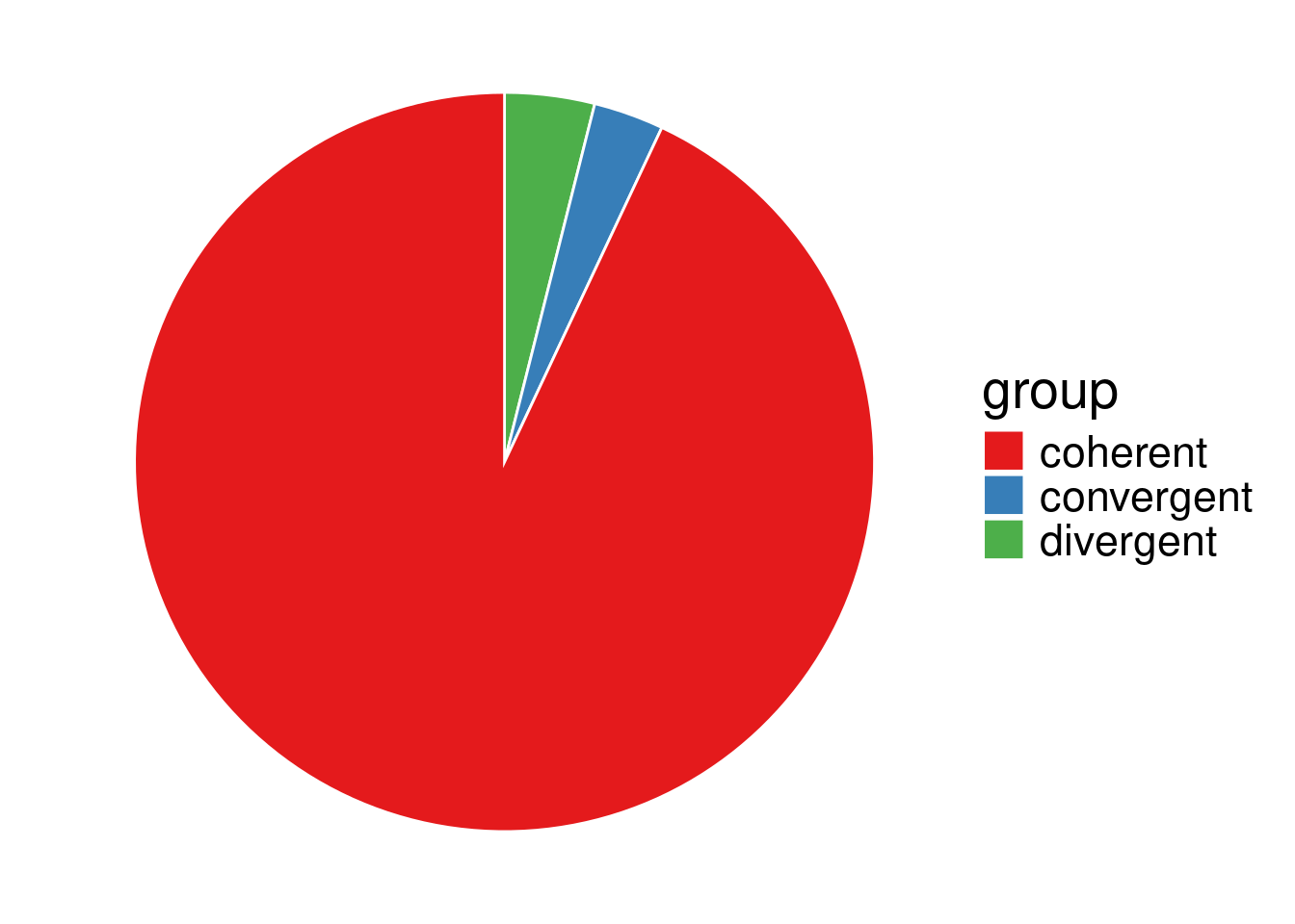
my_piechart(data_sp0)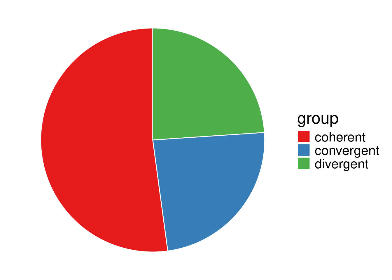
g_legend<-function(a.gplot){
  tmp <- ggplot_gtable(ggplot_build(a.gplot))
  leg <- which(sapply(tmp$grobs, function(x) x$name) == "guide-box")
  legend <- tmp$grobs[[leg]]
  return(legend)}
# Grid plot two by two for ggplot
p1 <- my_piechart(data_lp0)
mylegend<-g_legend(p1)
p2 <- my_piechart(data_sp0)

p1 <- p1 + ggtitle("Local pairs")
p2 <- p2 + ggtitle("Successive pairs")

p3 <- grid.arrange(arrangeGrob(p1 + theme(legend.position="none"),
                         p2 + theme(legend.position="none"),
                         nrow=1),
             mylegend, nrow=2,heights=c(10, 1))
p3TableGrob (2 x 1) "arrange": 2 grobs
z cells name grob
1 1 (1-1,1-1) arrange gtable[arrange]
2 2 (2-2,1-1) arrange gtable[guide-box]p1 <- my_piechart(data_lp0)
mylegend<-g_legend(p1)
p2 <- my_piechart(data_sp0)
p1 <- p1 + ggtitle("Local pairs")
p2 <- p2 + ggtitle("Successive pairs")
p3 <- grid.arrange(arrangeGrob(p1 + theme(legend.position="none"),
p2 + theme(legend.position="none"),
nrow=1),
mylegend, nrow=2,heights=c(10, 1))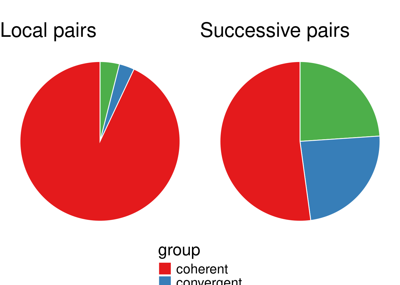
ggsave("media/plots/20240529_concordance_orientation_TAIR10.svg", p3, width = 10, height = 10)p <- plot_ly(data_sp0, labels=~group, values=~value, type="pie", textposition='outside', textinfo="label+percent")
p %>% layout(title = '',
xaxis = list(showgrid = FALSE, zeroline = FALSE, showticklabels = FALSE),
yaxis = list(showgrid = FALSE, zeroline = FALSE, showticklabels = FALSE))6.1.3 Statistical test
cf. Lê Hoang 2017
I will make the same test as Julie Lê-Hoang in its master internship report. In this report the following nomenclature is used:
- PST: Pair Successive TAG – sucessive pair of genes not separated by any spacer gene belonging to the same family
- PSnT: Pair Successive not TAG – successive pair of genes not seperated by any spacer gene not necessarilly belonging to the same family
The proposed test is a Fisher test on a contingency table.
Here is the shape of the count table, for no spacer (definition type of TAG0, or SP0)
| group | Coherent | Convergent | Divergent |
|---|---|---|---|
| PST (LP0) | \(a\) | \(b\) | \(c\) |
| PSnT (SP0) | \(d\) | \(e\) | \(f\) |
Hypotheses
\[ \begin{cases} (H_0) & \text{the proportion of each orientation concordance is similar between both groups} \\ (H_1) & \text{the proportion is different between PST and PSnT} \end{cases} \]
Test statistics
Using the notation in the contingency table above, the probability of the configuration, considering only two categories is defined as:
\[ p = \frac{\binom{a+b}{a} \binom{c + d}{c}}{\binom{n}{a+c}} \]
Here \(p\) corresponds to the \(p\)-value of the statistical test. (?)
In our case, however, the contingency table is not 2x2 so we cannot simply apply this exact formula based hypergeometric distribution presented above. The R implementation in fisher.test uses the Mehta and Patel network algorithm (cf. https://doi.org/10.2307/2288652/ )
head(data_lp0) group value
1 coherent 1516
2 convergent 50
3 divergent 64head(data_sp0) group value
1 coherent 14014
2 convergent 6429
3 divergent 6432nb. In a contingency table, the effective have to be independent. In our case, the count for SP0 includes the count of LP0 (a gene pair that do not necessarilly belong to the same family, can however belong to the same family), so to get the count for ‘non TAG’ gene pairs, we have to substract the LP0 counts from the SP0 ones.
contingency_table <- as.data.frame(t(data_lp0))
columns <- contingency_table[1,]
contingency_table <- contingency_table[-1,]
contingency_table <- mutate_all(contingency_table, function(x) as.numeric(x)) # I lost the numeric time doing my cooking
colnames(contingency_table) <- columns
contingency_table <- rbind(contingency_table, data_sp0[,2] - contingency_table[,1])
rownames(contingency_table) <- c("LP0", "SP0")
contingency_table
coherent convergent divergent
LP0 1516 50 64
SP0 12498 4913 4916With the following command, I get the error below.
fisher.test(contingency_table)Error in fisher.test(x) :
FEXACT error 6 (f5xact). LDKEY=443 is too small for this problem: kval=33989596.
Try increasing the size of the workspace.As reported by Julie, I have to increase the workspace size:
fisher.test(contingency_table, workspace=2e+06)
    Fisher's Exact Test for Count Data

data:  contingency_table
p-value < 2.2e-16
alternative hypothesis: two.sided
Conclusion
\(2.2\cdot 10^{-16} < 0.05\), so at level \(\alpha = 0.05\), we reject \((H_0)\), the proportion of convergent, coherent and divergent orientations of adjacent gene pairs significantly differs depending on whether the gene pair belongs to the same family (LP0) or not (SC0), as expected from a sight on the pie charts. In particular, convergent gene orientation tends to be over-represented among adjacent gene pairs belonging to the same family, compared to gene pairs belonging to different families.
6.2 For other definitions
Info: This workflow output uses the TAIR10_pep_20101214 file, as defined in exp/mutual/config/TAIR10_LêHoang_jeu1.yaml. It aims at using the same tool configuration as reported in Julie’s report (except the filtering of mitochondrial and chloroplastic genes, for now).
tair10_features_df_2 <- read.table("exp/mutual/results/bak/2024-06-03/ifb/TAIR10_LêHoang_jeu1_features.tsv", sep = "\t")
colnames(tair10_features_df_2) <- c("name", "chromosome", "strand", "start", "end", "type")
tair10_features_df_2 <- tair10_features_df_2[tair10_features_df_2$type == "gene",]
head(tair10_features_df_2)
name chromosome strand start end type
2 AT1G01010 Chr1 1 3631 5899 gene
3 AT1G01020 Chr1 -1 5928 8737 gene
4 AT1G01030 Chr1 -1 11649 13714 gene
5 AT1G01040 Chr1 1 23146 31227 gene
6 AT1G01046 Chr1 1 28500 28706 gene
8 AT1G01050 Chr1 -1 31170 33153 genetair10_local_pairs_df_2 <- read.table("exp/mutual/results/bak/2024-06-03/ifb/lists/TAIR10_LêHoang_jeu1/local_gene_pairs.tsv", header=TRUE, sep = "\t")
head(tair10_local_pairs_df_2) gene_a gene_b definition
1 AT1G01580 AT1G01590 LP0
2 AT1G02190 AT1G02205 LP0
3 AT1G02220 AT1G02230 LP0
4 AT1G02230 AT1G02250 LP0
5 AT1G02300 AT1G02305 LP0
6 AT1G02430 AT1G02440 LP0tair10_successive_pairs_df_2 <- read.table("exp/mutual/results/bak/2024-06-03/ifb/lists/TAIR10_LêHoang_jeu1/successive_gene_pairs.tsv", header=TRUE, sep = "\t")
head(tair10_successive_pairs_df_2) gene_a gene_b definition
1 AT1G01010 AT1G01020 SP0
2 AT1G01020 AT1G01030 SP0
3 AT1G01030 AT1G01040 SP0
4 AT1G01040 AT1G01046 SP0
5 AT1G01050 AT1G01060 SP0
6 AT1G01060 AT1G01070 SP0How many definition do I have?
unique(tair10_local_pairs_df_2[,"definition"])[1] "LP0" "LP1" "LP5" "LP10"unique(tair10_successive_pairs_df_2[,"definition"])[1] "SP0" "SP1" "SP5" "SP10"Sanity check: Let’s first check we get the same conclusion with 0 spacer on this dataset.
definition <- 0local_definition_column <- paste0("LP", definition)
sp_definition_column <- paste0("SP", definition)local0_2 <- tair10_local_pairs_df_2[tair10_local_pairs_df_2[,"definition"] == local_definition_column,]
successive0_2 <- tair10_successive_pairs_df_2[tair10_successive_pairs_df_2[,"definition"] == sp_definition_column,]convergence_local0_2 <- apply(local0_2[,c("gene_a", "gene_b")], 1, function(row) get_convergence(row, tair10_features_df_2))
convergence_successive0_2 <- apply(successive0_2[,c("gene_a", "gene_b")], 1, function(row) get_convergence(row, tair10_features_df_2))data_lp0_2 <- as.data.frame(table(convergence_local0_2)) %>% rename(., value=Freq, group=convergence_local0_2)data_sp0_2 <- as.data.frame(table(convergence_successive0_2)) %>% rename(., value=Freq, group=convergence_successive0_2)my_piechart(data_lp0_2) + ggtitle("Local pairs LP0 (2)")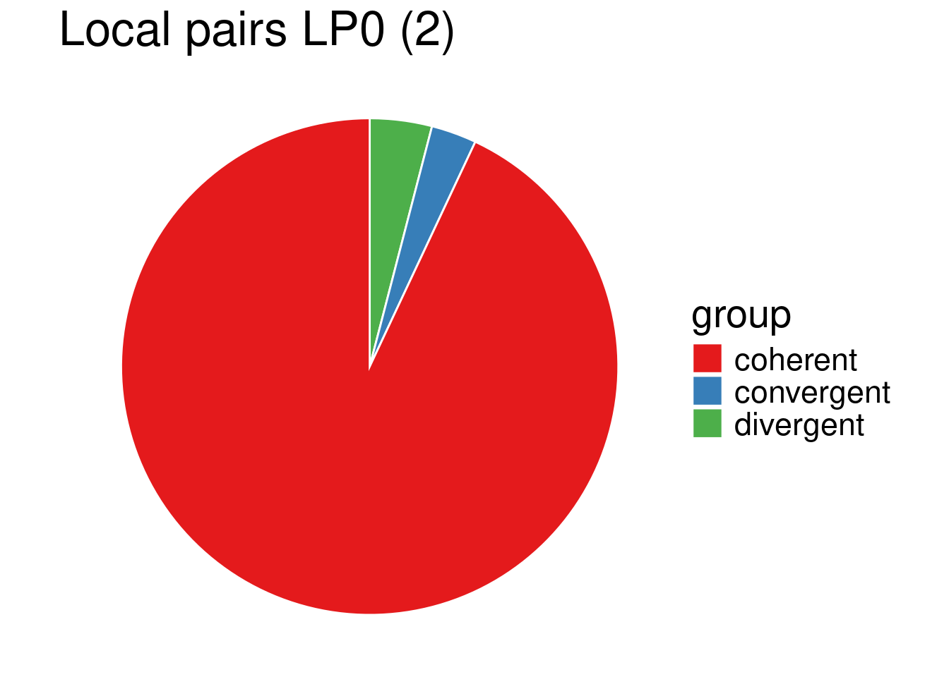
my_piechart(data_sp0_2) + ggtitle("Successive pairs SC0 (2)")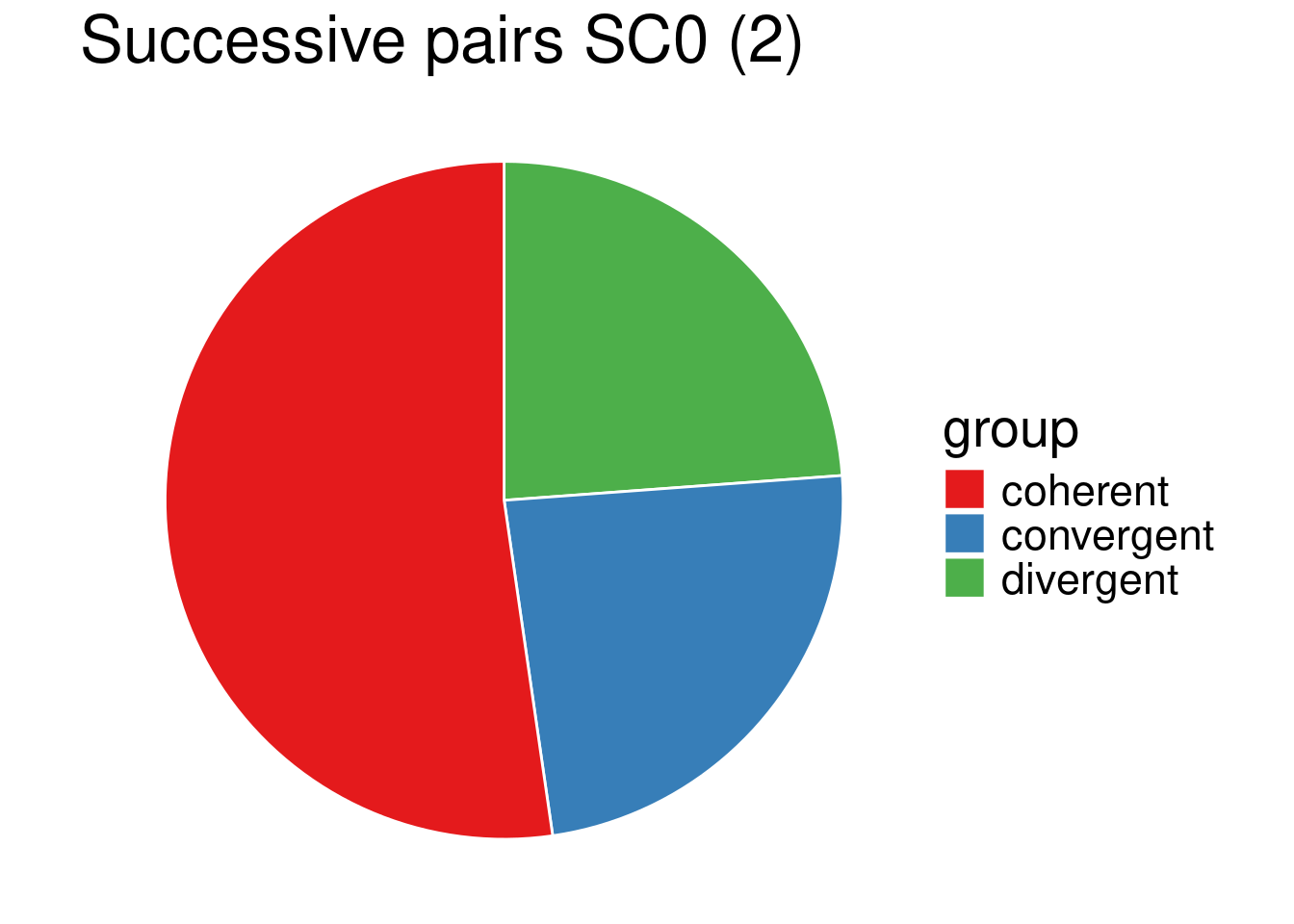
#' Construct the contingency table
#' @param data_1 a dataframe containing the count of the first column of the contingency table, in its first row
#' @param data_all a dataframe containing marginal count of the contingency table, in its first row
#' @param names a vector with row names (data_1 group and data_all - data_1 corresponding group)
#' @return a 2xc numeric matrix, with two rows, a row for each group, and c columns corresponding to each condition
get_contingency_table <- function(data_1, data_all, names=c("LP0", "SP0")) {
contingency_table <- as.data.frame(t(data_1))
columns <- contingency_table[1,]
contingency_table <- contingency_table[-1,]
contingency_table <- mutate_all(contingency_table, function(x) as.numeric(x)) # I lost the numeric time doing my cooking
colnames(contingency_table) <- columns
contingency_table <- rbind(contingency_table, data_all[,2] - contingency_table[,1])
rownames(contingency_table) <- names
contingency_table
}contingency_table_2_0 <- get_contingency_table(data_lp0_2, data_sp0_2, names=c("LP0", "SP0"))
contingency_table_2_0 coherent convergent divergent
LP0 1452 46 63
SP0 12844 5076 5064Fisher test, for the concordance of gene orientation proportion discrepancies between adjacent genes in the same family and adjacent genes in different families, for the data set reproduced from Julie Lê Hoang 2017:
fisher.test(contingency_table_2_0, workspace = 2e+06)
Fisher's Exact Test for Count Data
data: contingency_table_2_0
p-value < 2.2e-16
alternative hypothesis: two.sidedWe have the same conclusion.
6.2.1 How does this proportion in TAG evolve as the number of spacer increases?
save <- FALSEdata_lp_def <- list()
data_sp_def <- list()
definitions <- c(0, 1, 5, 10)
for (definition in definitions) {
local_definition_column <- paste0("LP", definition)
sp_definition_column <- paste0("SP", definition)
local_pairs <- tair10_local_pairs_df_2[tair10_local_pairs_df_2[,"definition"] == local_definition_column,]
successive_pairs <- tair10_successive_pairs_df_2[tair10_successive_pairs_df_2[,"definition"] == sp_definition_column,]
convergence_local <- apply(local_pairs[,c("gene_a", "gene_b")], 1, function(row) get_convergence(row, tair10_features_df_2))
convergence_successive <- apply(successive_pairs[,c("gene_a", "gene_b")], 1, function(row) get_convergence(row, tair10_features_df_2))
data_local <- as.data.frame(table(convergence_local)) %>% rename(., value=Freq, group=convergence_local)
data_successive <- as.data.frame(table(convergence_successive)) %>% rename(., value=Freq, group=convergence_successive)
if (save) {
write.table(convergence_local, paste0("tmp/R/convergence_TAIR10_LêHoang_jeu1.LP", definition, ".tsv"))
write.table(convergence_successive, paste0("tmp/R/convergence_TAIR10_LêHoang_jeu1.SP", definition, ".tsv"))
}
data_lp_def <- append(data_lp_def, list(data_local))
data_sp_def <- append(data_sp_def, list(data_successive))
}Let plot the pie chart of all definition.
# Use two columns: one for Local Pairs and the other for Successive Pairs
# Then each row is the definition in ascending order
p <- list()
i <- 1
for (index in seq_along(definitions)) {
  definition <- definitions[index]
    data <- data_lp_def[[index]]
    name <- paste0("LP", definition)
  p[[i]] <- my_piechart(data) + ggtitle(name) + theme(legend.position="none")
  i <- i + 1
   data <- data_sp_def[[index]]
    name <- paste0("SP", definition)
  p[[i]] <- my_piechart(data) + ggtitle(name) + theme(legend.position="none")
  i <- i + 1
}

grid.arrange(grobs=p, ncol=2)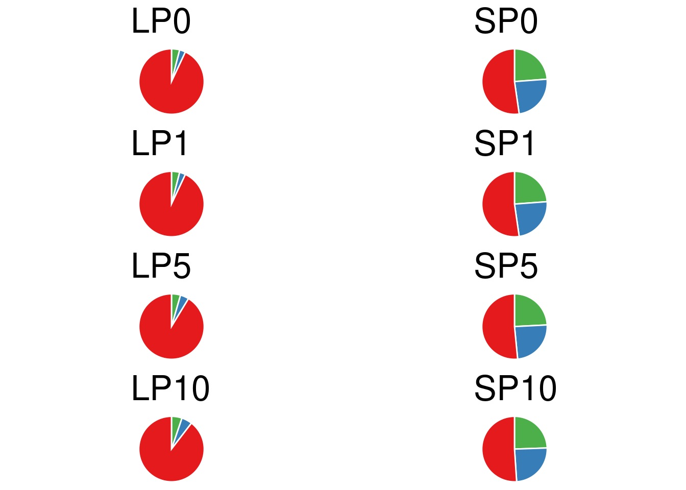
6.2.2 Contingency tables
contingency_tables <- list()
for (i in seq_along(definitions)) {
  definition <- definitions[i]
  data_lp <- data_lp_def[[i]]
  data_sp <- data_sp_def[[i]]
  contingency_table <- get_contingency_table(data_lp, data_sp, names=paste0(c("LP", "SP"), definition))
  contingency_tables <- append(contingency_tables, list(contingency_table))
  print(contingency_table)
}
coherent convergent divergent
LP0 1452 46 63
SP0 12844 5076 5064
coherent convergent divergent
LP1 1452 46 63
SP1 12844 5076 5064
coherent convergent divergent
LP5 3210 149 157
SP5 67105 29883 29815
coherent convergent divergent
LP10 3813 223 222
SP10 135287 62882 62855fisher.p.values <- lapply(contingency_tables, function(table) fisher.test(table, workspace=2e+07)$p)library(scales)
ggplot() + geom_point(mapping=aes(x=definitions, y=as.numeric(fisher.p.values))) + scale_x_continuous(breaks=breaks_pretty())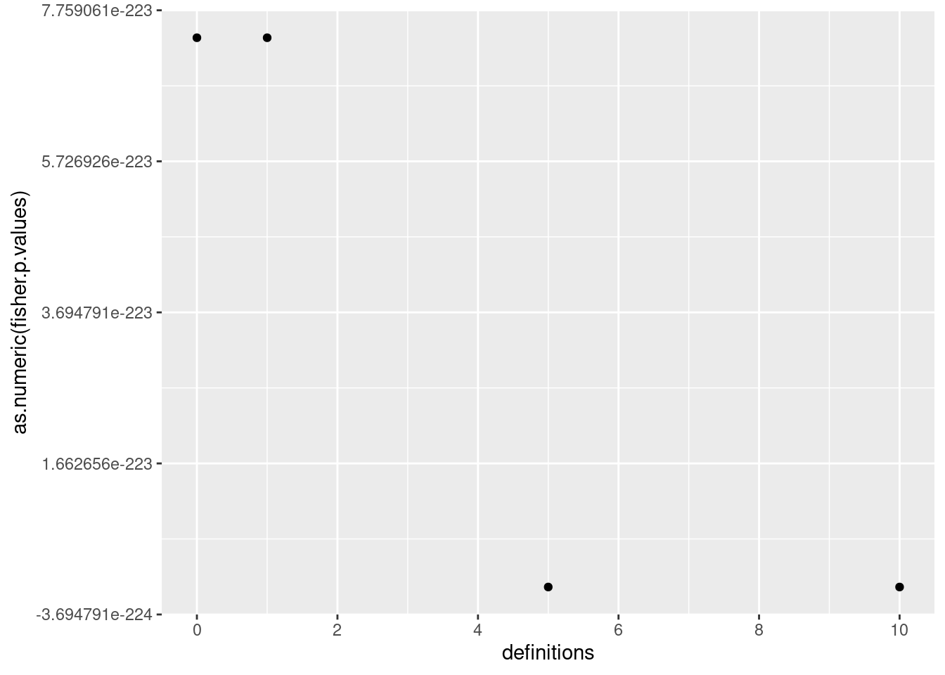
plot(definitions, fisher.p.values)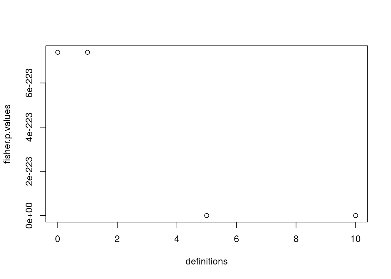
6.3 References
Wikipedia contributors. (2024, February 28). Fisher’s exact test. In Wikipedia, The Free Encyclopedia. Retrieved 07:57, June 3, 2024, from https://en.wikipedia.org/w/index.php?title=Fisher%27s_exact_test&oldid=1210712147
https://lemakistatheux.wordpress.com/tag/le-test-de-fisher-freeman-halton/